Starting in 2004, we began to apply the transient grating techniques developed by Nuh Gedik in an entirely different context, the dynamics of spins in semiconductors.  Transient grating measurements of spin diffusion in undoped semiconductors had been demonstrated by the group of Alan Miller at the University of St. Andrews.  In our research we use the added sensitivity of coherent heterodyne detection to study spin propagation is doped semiconductors.  We measure spin dynamics in the two-dimensional electron gas as a function of electron density, dimensionality, and strengh of spin-orbit interactions.  Our research in this area has benefitted greatly from close collaboration with the groups of David Awschalom at UC Santa Barbara and Shoucheng Zhang at Stanford University.

Transient spin gratings

All of these measurements are based on the optical orientation effect in zincblende semiconductors.  In semiconductors with the zincblende structure, optical excitation with circularly polarized light injects an electron with definite spin into the conduction band.  That is, left-circular light injects spin up and right circular injects spin down.  The trick developed by Cameron et al. was to excite the sample with a pair of pump beams with orthogonal linear polarization.  The interference of such beams leads to a modulation of the photon helicity , rather than the optical intensity, as in the conventional transient grating experiment.   Because of the optical orientation efffect, the modulation of photon helicity leads to modulation of electron spin polarization, as shown below, in a sketch from  Cameron et al.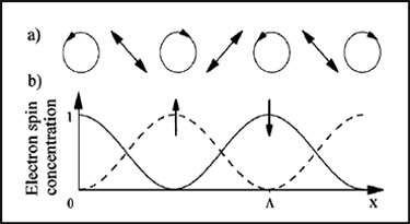

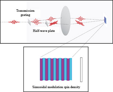
A cartoon sketch of how we implement this experiment is shown below.  Pulses from the Ti:Saphhire laser are split using a transmission grating.  (For more details on the coherent detection technique go to “Optical Techniques.”) One of the two beams goes to a half-wave plate that rotates the plane of polarization by 90°.  Mirrors (rather than the lens shown below) are used to focus the two beams onto a single spot on the sample.  The color plot illustrates the resulting modulation of electron spin density.

Essentially complete information about the q-dependent spin time dynamics is contained in the time-evolution of the transient spin grating following its creation at time t=0.  We measure this time-evolution using a pair of orthogonally polarized probe-beams.  Each of these beams has components that are transmitted through, and diffracted by, the spin grating.   See “Optical techniques” for an explanation of how the these beams are used to probe the amplitude and phase of the spin-density modulation.

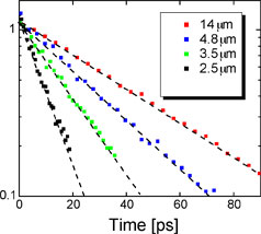
Decay of spin polarization at room temperature for different grating wavevectors

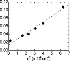
Spin grating decay rate γ plotted versus square of grating wavevector

The plots above show typical results at room temperature for the 2DEG in GaAs/GaAlAs quantum wells.  At each wavevector the decay of the grating is a simple exponential.  A plot of the decay rate γ vs. q2  yields a straight line with nonzero y-axis intercept.  The slope of the line yields Ds, the spin diffusion coefficient, and the intercept yields τs, the spin relaxation rate.

Far-infrared spectroscopy of multiferroics

In our first studies we measured Ds as a function of temperature and carrier concentration in several quantum well samples.  We compared Ds obtained from the spin grating with the charge diffusion coefficient Dc measured using transport methods by the Awshalom group on the same set of samples.  We discovered that the two coefficients were very different with Ds significantly smaller than Dc.  The panel on the left shows a comparison of spin and charge diffusion coefficients for three quantum well samples of different density.  The solid lines are Dc and the solid circles are Ds.. The red lines are the predictions of the spin Coulomb drag theory of Giovanni Vignale and Irene D’Amico.  The insets show the ratio of spin to charge diffusion rates.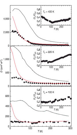

As the agreement between theory and experiment bears out, we had (inadvertently!) made the first observation an effect known as spin Coulomb drag, predicted in the late ‘90’s by Vignale and D’Amico.

Spin Coulomb drag is the intrinsic friction experienced by down-spin electrons as they attempt to flow past up-spin electrons, and vice versa.  The cartoon above illustrates the physical origin of the difference between spin and charge propagation.  Two electrons with opposite spin approach each other on the left hand side of the sketch.  Before the collision there charge current is oriented to the right (let’s ignore the convention that the electronic charge is negative for the moment!) and the net spin current is in the vertical direction (or towards the top of the page).  The collision conserves the total momentum of the two electrons, and thus the charge current they carry, Jc, is unchanged.  However the total spin current, Jspin, carried by electrons of opposite spin is proportional to their relative momentum, which will change as momentum is exchanged during the collision.  For the collision shown in the cartoon the spin current is towards the bottom of the page after the collision. The microscopic process of such singlet state collisions corresponds to a macroscopic frictional force, the “spin-Coulomb drag,” that inhibits the relative motion of electrons with opposite spin.

Depending on the application, spin Coulomb drag could prove to be either an advantage or a disadvantage. Although the drag adds to the force required to drive a pure spin current, it will extend the lifetime of localized packets of polarized spin that could be used to store and transmit information.

Searching for the Persistent Spin Helix

Following the discovery of spin-Coulomb drag, we began investigating the effects of spin-orbit coupling on spin diffusion.  Spin-orbit coupling plays a crucial role in spin-based electronics (or spintronics).  It provides a mechanism for controlling the spin state of electrons through electric rather than magnetic fields.  However, spin-orbit coupling also has the unwanted effect of causing spin relaxation, or loss of spin memory.  In the past year we proposed, and experimentally verified, a new mechanism for extending spin memory time in the presence of spin-orbit coupling.  We showed that in the presence of spin-orbit coupling of a certain symmetry an inhomogenous spin distribution in the form of a spin helix or cycloid can have an infinite lifetime. 

If you’re like me, the very sound of “spin-orbit coupling” provokes a shudder, bringing back memories of torments such as “Clebsch-Gordon coefficients.”  However, spin-orbit in the 2DEG (formed in a GaAs quantum well) has a form that is easy to visualize.  The spin-orbit term in the Hamiltonion is equivalent to an inplane magnetic field, albeit one that depends on the electron’s wavevector, k.  The coupling comes in two symmetry flavors, known as Rashba and Dresselhaus.  Vector field plots that help to visualize these effective magnetic fields are shown below:

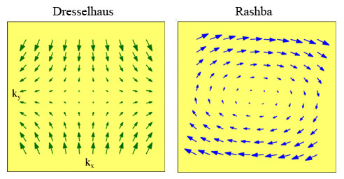The Dresselhaus term, shown on the left, results from the breaking of inversion symmetry that is intrinsic to the crystal structure of GaAs.  The Rashba term, illustrated on the right.

The spin of an electron in a k-state will precess at a rate determined the effective spin-orbit field.  For GaAs quantum wells the typical precession frequency is of order 50 GHz.  Left on its own, the spin of an electron will flip on a time scale of 10 ps.  Somewhat paradoxically, the lifetime becomes longer in the presence of scattering, which interrupts the free precession.  The disorientation of the spin due to interrupted free-precession is known as Dyakanov-Perel spin relaxation.  At room temperature the typical DP relaxation time for an n-doped GaAs quantum well is of order 100 ps.

The time quoted above is the how long it takes for a spatially uniform spin polarization of the electron sea to relax to zero.  As a result of our spin grating experiments, we became interested in the question of how this lifetime changes for a spatially inhomogeneous spin polarization.  The “naïve” view would be that the decay rate of the grating would be the sum of the DP rate and the rate governed by spin diffusion.  That is,

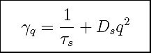where γq is the decay rate of a spin polarization wave with wavevector q .  In fact, this simple behavior is exactly what we, and Cameron et al. had observed at room temperature.

In 2002, a very stimulating paper appeared, by Nunez, Burkov, and MacDonald (NBM), reporting theoretical predictions for the decay rate of periodic spatial distributions of spin polarization (of the kind that we can generate in our transient grating experiment).  Their calculations were based on a Hamiltonian that contained only the Rashba term.

The graph below, on which we plot spin polarization lifetime as a function of wavevector, illustrates some of the predictions.  The blue curve is the “naïve” expectation for the lifetime, simply the reciprocal of the formula for γq that has been given above.  This plot agrees with our expectation that diffusion wipes out spin polarization waves more rapidly as their wavelength gets shorter.   The red curve is generated from the formulas derived by NBM, indicating instead that spin polarization lifetime reaches a maximum at nonzero wavevector .  Somehow the effect of spin propagation is to preserve, rather than destroy, the spin polarization state.  How can this be?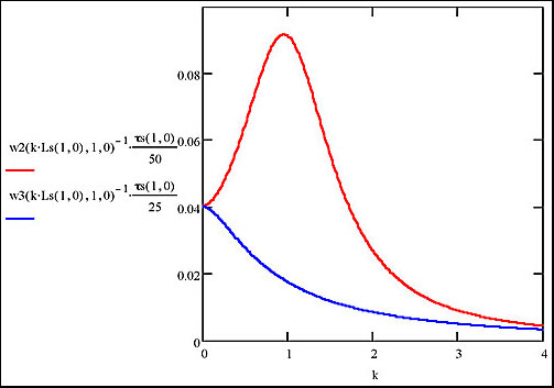

To understand the physical origin of this effect, we consider a 1D version of this problem.  Imagine an electron confined to move on a line, with a spin that precesses only in a plane that contains this line.  In such a situation, the net change in spin direction of the electron depends only on its net displacement, and not how it was scattered on its way from point A to point B.   We can define a spin diffusion length, Ls,as the displacement that leads to a precession through an angle of 2π.  It is clear that in this system a spin polarization wave with wavelength Ls, will live forever.  As the electron propagates its spin will continue to point in the direction of the initial spin polarization.

Now that we understand the infinite lifetime predicted for 1D, what about the rather modest enhancement predicted by NBM for 2D?  As the plots illustrate, the peak lifetime in the NBM model is about a factor of seven longer than the naïve diffusion model, and seven is a far cry from infinity.  The reason that the peak lifetime is finite in 2D is that the perfect correlation between displacement and precession gets screwed up (to use the scientific term).   The net change in spin direction is not a function simply of the net displacement, rather it depends on the path that the electron takes to get from point A to point B.  However, the spin-space/real-space correlations are not completely destroyed and the imperfect correlation results in the finite but enhanced spin polarization lifetime.

Now it can be told: the Rashba + Dresselhaus story

To tell the truth, the goal of our initial transient spin grating experiments was to observe the spin grating lifetime enhancement predicted by NBM.  To our surprise, the results were closer to the naïve spin diffusion model than to NBM.  This was not a total loss as we did observe the spin Coulomb drag.  However we were left with a mystery as to why the NBM effect was “missing.”

When we finally found the NBM effect, it turned out to be in the last place we looked (how often it turns out this way!).  Rotating the sample by 90°, orienting q parallel to the direction, produced a dramatic change in the decay dynamics of the spin grating, as shown below left: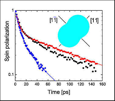  

For our original orientation, the spin grating decay is very close to single exponential.  For the “new” orientation, the decay is clearly biexponential, and the two exponential components have approximately equal weight.

These observations led very rapidly to a greater understanding of our samples and of the spin propagation dynamics.  We recognized that the strong anisotropy comes from the presence of a Rashba term that is present despite of the nominal symmetry of our wells.   Our Stanford theoretician collaborators, Shoucheng Zhang and Andrei Bernevig, were able to generalize the NBM calculation the presence of both Rashba and Dresselhaus terms.  To our surprise, even a relatively small admixture of Rashba coupling creates the large anisotropy that we observed.  Considering Rashba and Dresselhaus terms together led to an even more interesting and unexpected conclusion.

Samples with equal Rashba and Dresselhaus coupling are special.

The calculations of Bernevig and Zhang showed that when Rashba=Dresselhaus (or a=b in the standard notation) the lifetime of the spin grating with q~ 1/Ls diverges, just as it does in one dimension.  The reason for the divergence can also be understood in a similar way to the 1D version.  When a=b the net precession of the electron’s spin depends only on its net displacement in the 11 direction.  In this case a spin helix (or more properly cycloid) with the “magic wavevector” will live forever.

Further details on both theory and experiment of the persistent spin helix can be found here.